AI Podcast
119 episodes — 90-second audio overviews on ai podcast.
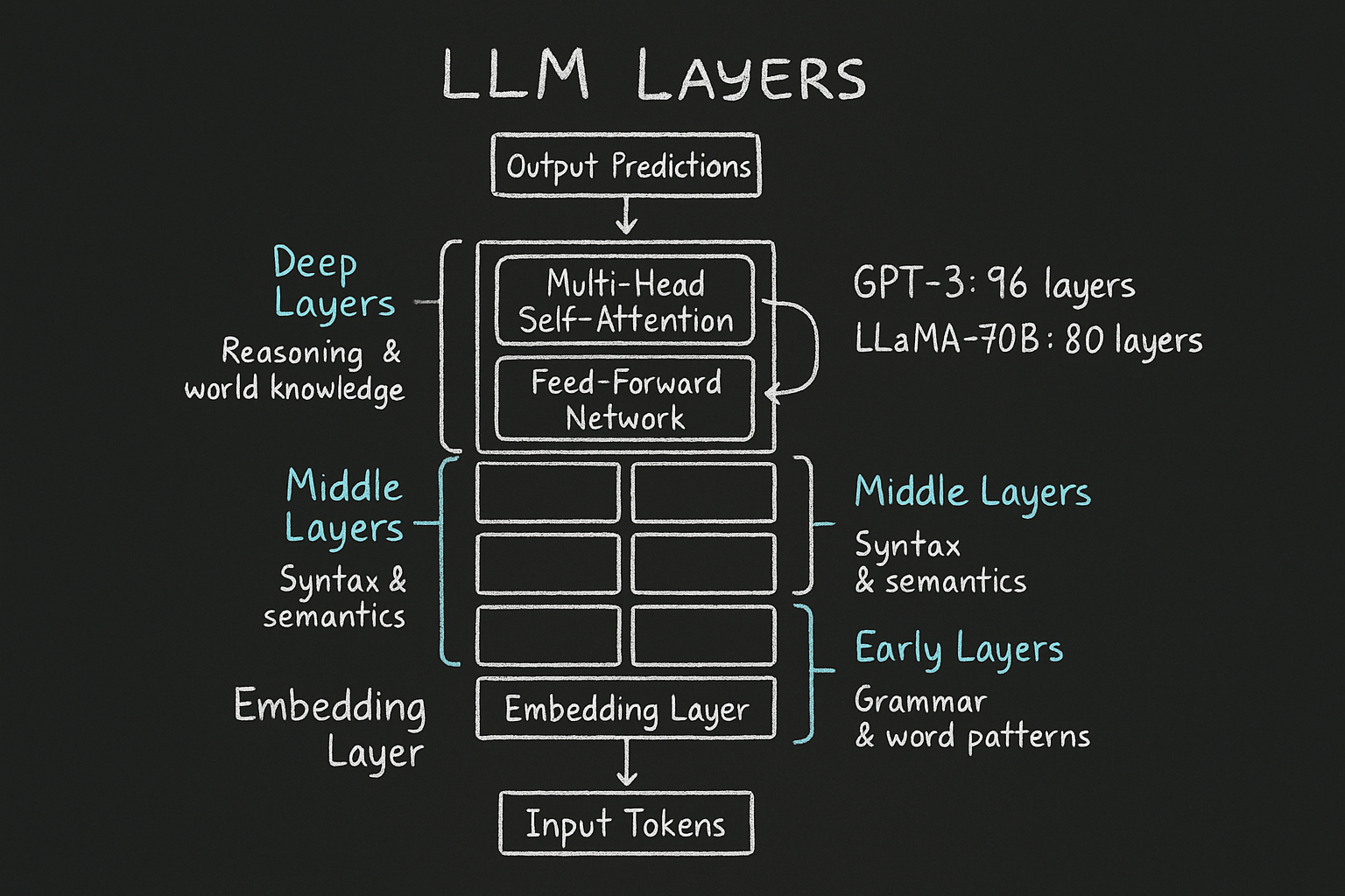
LLM layers — architecture of a large language model
A large language model is a deep stack of identical Transformer layers: early layers capture grammar, middle layers grasp semantics, and deep layers handle reasoning and world knowledge.
ControlNet — adding spatial conditioning
Injecting structural control signals (edge maps, human poses, depth maps) alongside text prompts for precise spatial layout control over the generated image.

Classifier-free guidance (CFG) — controlling prompt adherence
Blending conditional (text-guided) and unconditional predictions during generation; higher CFG values follow the text prompt more strictly at the cost of diversity.
CLIP guidance — text-image alignment for generation
OpenAI's CLIP model provides a shared text-image embedding space that steers the diffusion process toward images matching a text description.
Diffusion Transformers (DiT) — replacing U-Net with transformers
Using transformer blocks instead of U-Net for the denoising network — powers Sora, Flux, and SD3, offering better scaling and quality at large sizes.
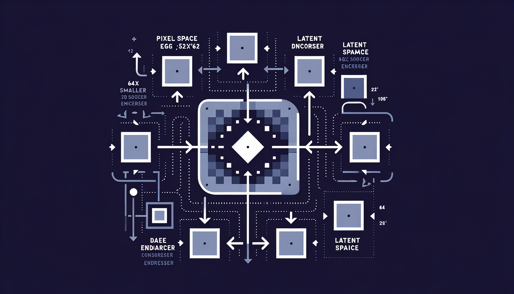
Latent diffusion — diffusing in compressed space
Running the diffusion process in a VAE's latent space (64x smaller than pixel space) rather than on raw pixels, making generation fast and memory-efficient.
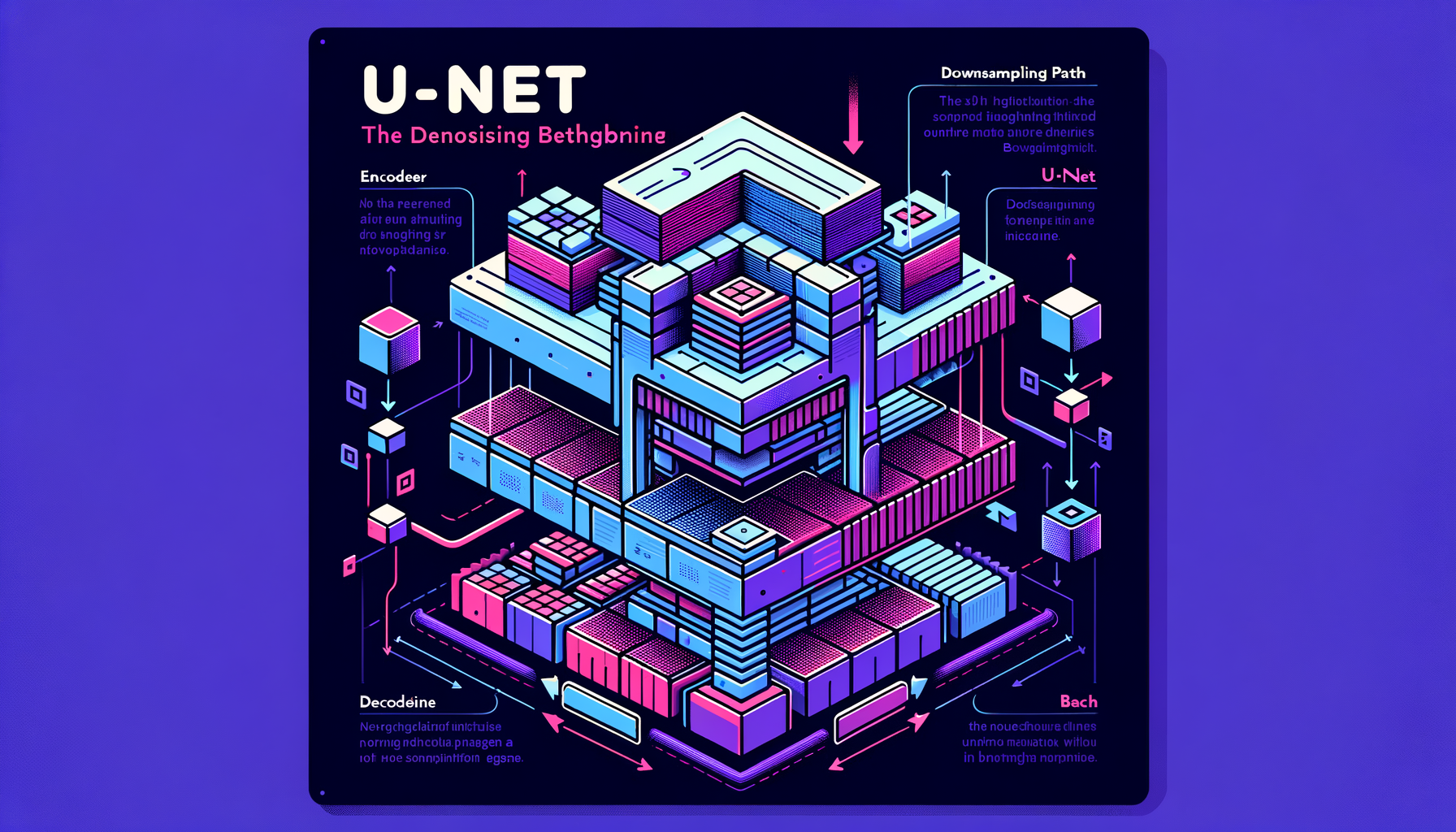
U-Net — the denoising backbone
An encoder-decoder convolutional network with skip connections that predicts the noise to remove at each diffusion step — the workhorse architecture of Stable Diffusion 1.x and 2.x.

Noise schedules — controlling how noise is added
Linear, cosine, or learned schedules define how much noise is injected at each of the T timesteps — directly impacting generation quality and training stability.
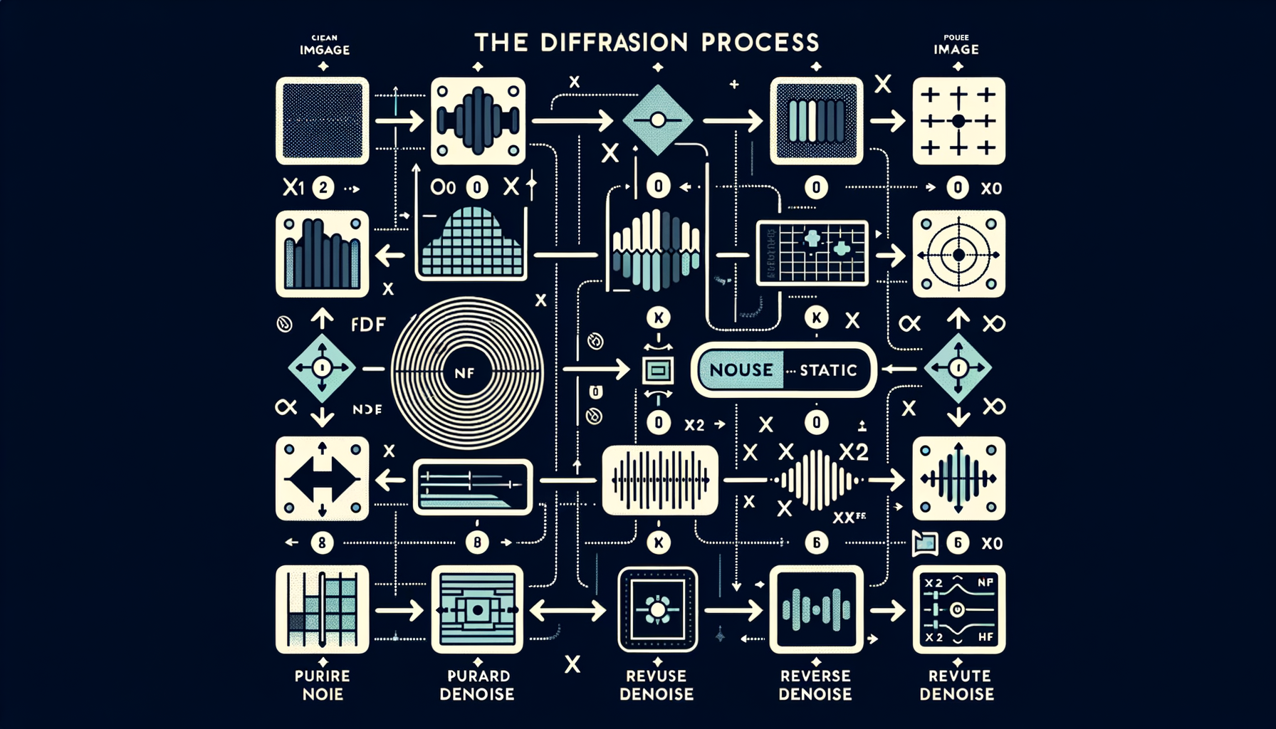
The diffusion process — forward noise, reverse denoise
Forward process: gradually add Gaussian noise over many steps until the image becomes pure static. Reverse process: learn to undo each step, recovering a clean image.
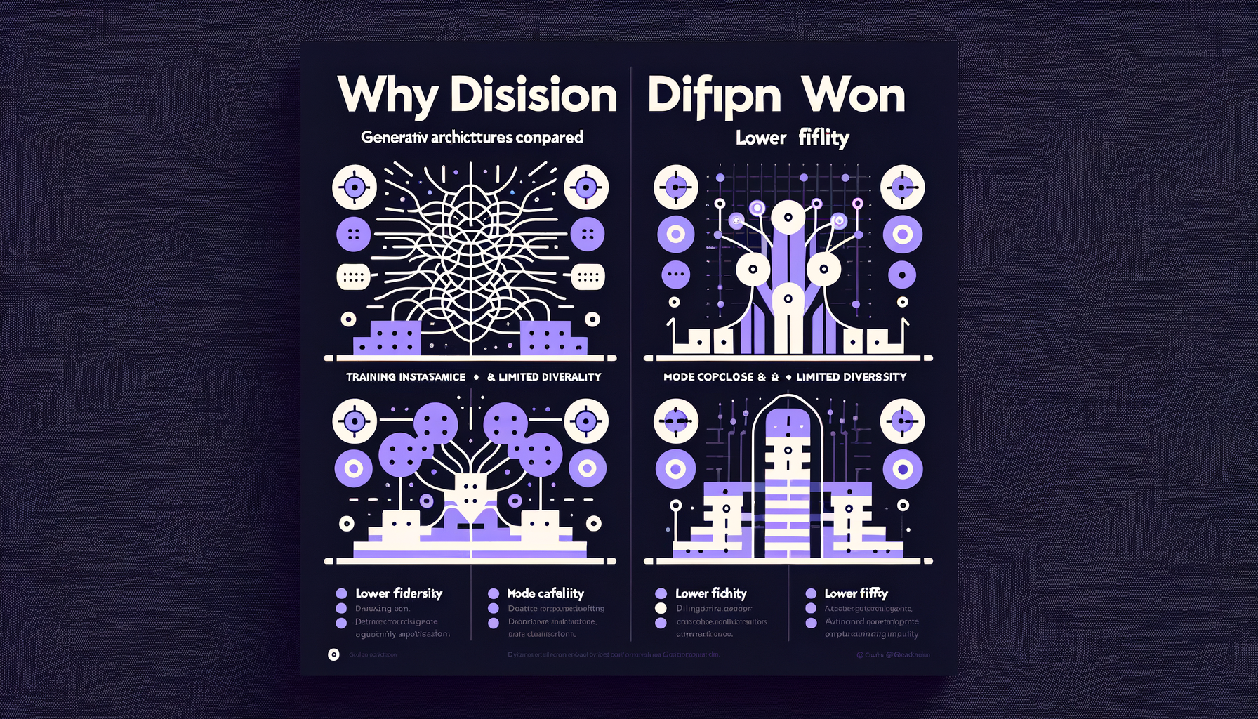
Why diffusion won — comparing generative architectures
Diffusion models offer stable training, mode coverage, better diversity, and higher fidelity than GANs, which is why they replaced GANs as the dominant approach for image and video generation.
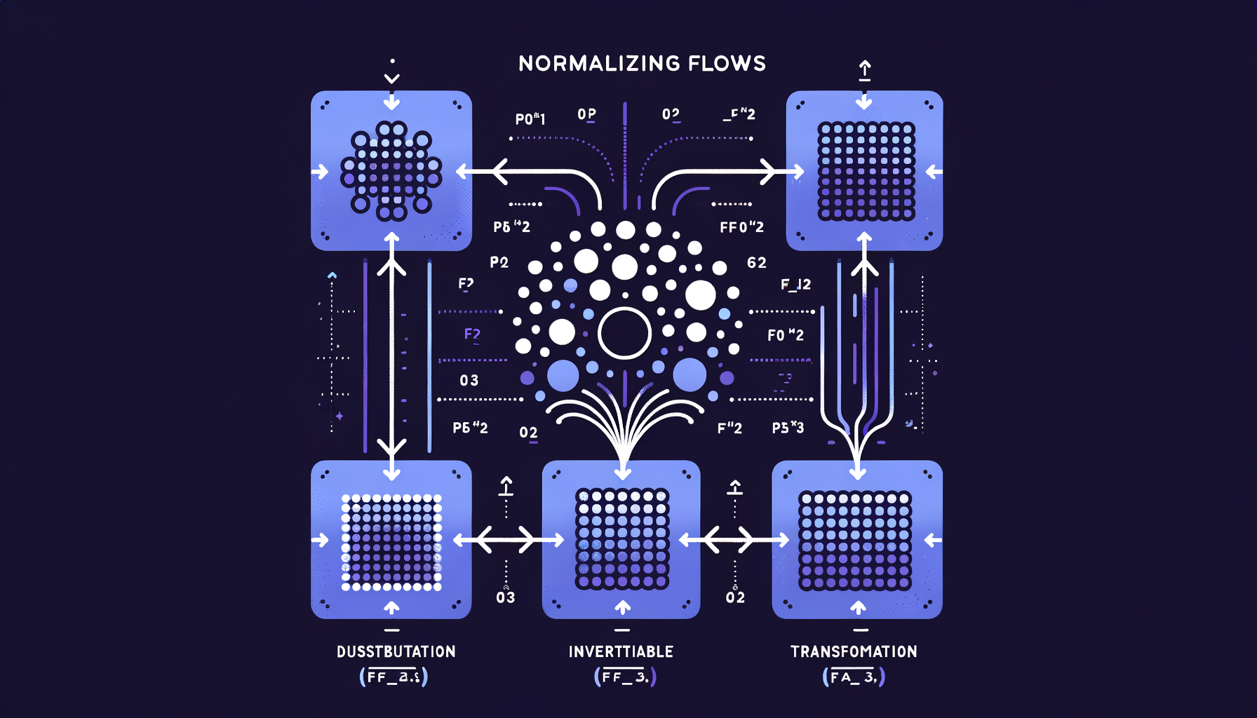
Normalizing Flows — invertible generation with exact likelihoods
Chains of invertible mathematical transformations that map simple distributions to complex ones, offering exact probability computation unlike GANs or VAEs.
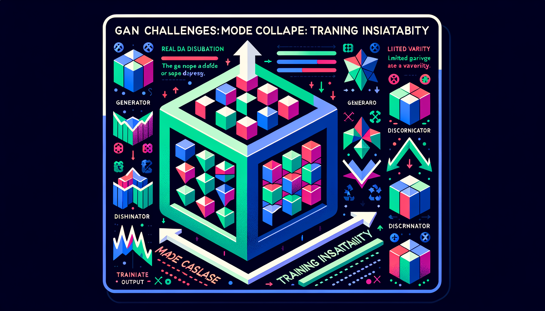
GAN challenges — mode collapse and training instability
GANs are notoriously difficult to train: the generator may produce limited variety (mode collapse), and the adversarial balance is fragile and sensitive to hyperparameters.
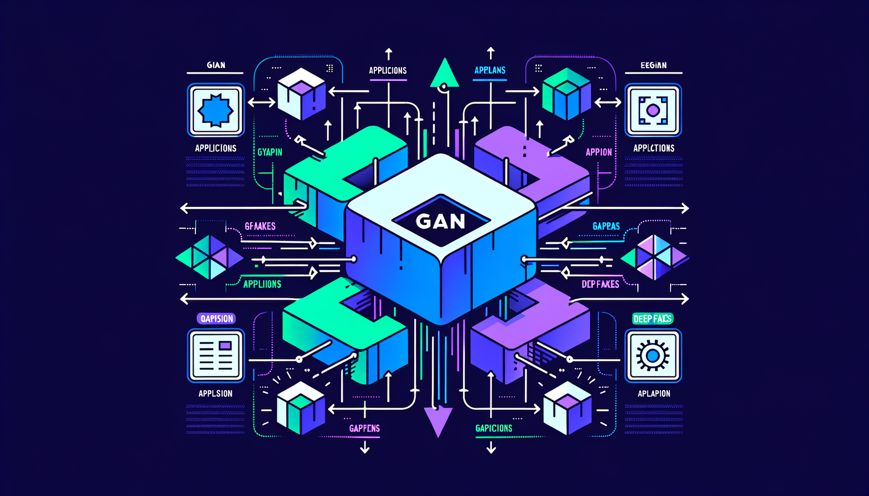
GAN applications — StyleGAN, deepfakes, super-resolution
GANs powered photorealistic face generation (StyleGAN), image enhancement (ESRGAN), and synthetic media — the dominant GenAI paradigm before diffusion.
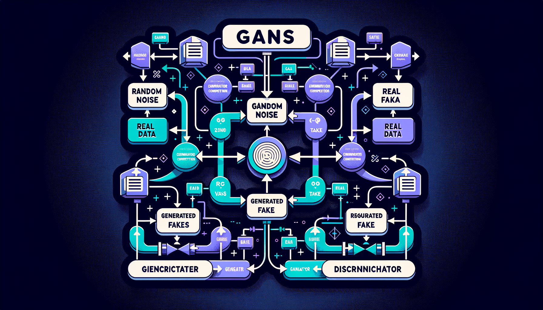
GANs — generator vs discriminator competition
Two networks in adversarial training: a generator creates fakes, a discriminator detects them — the competition drives both to improve, producing increasingly realistic outputs.
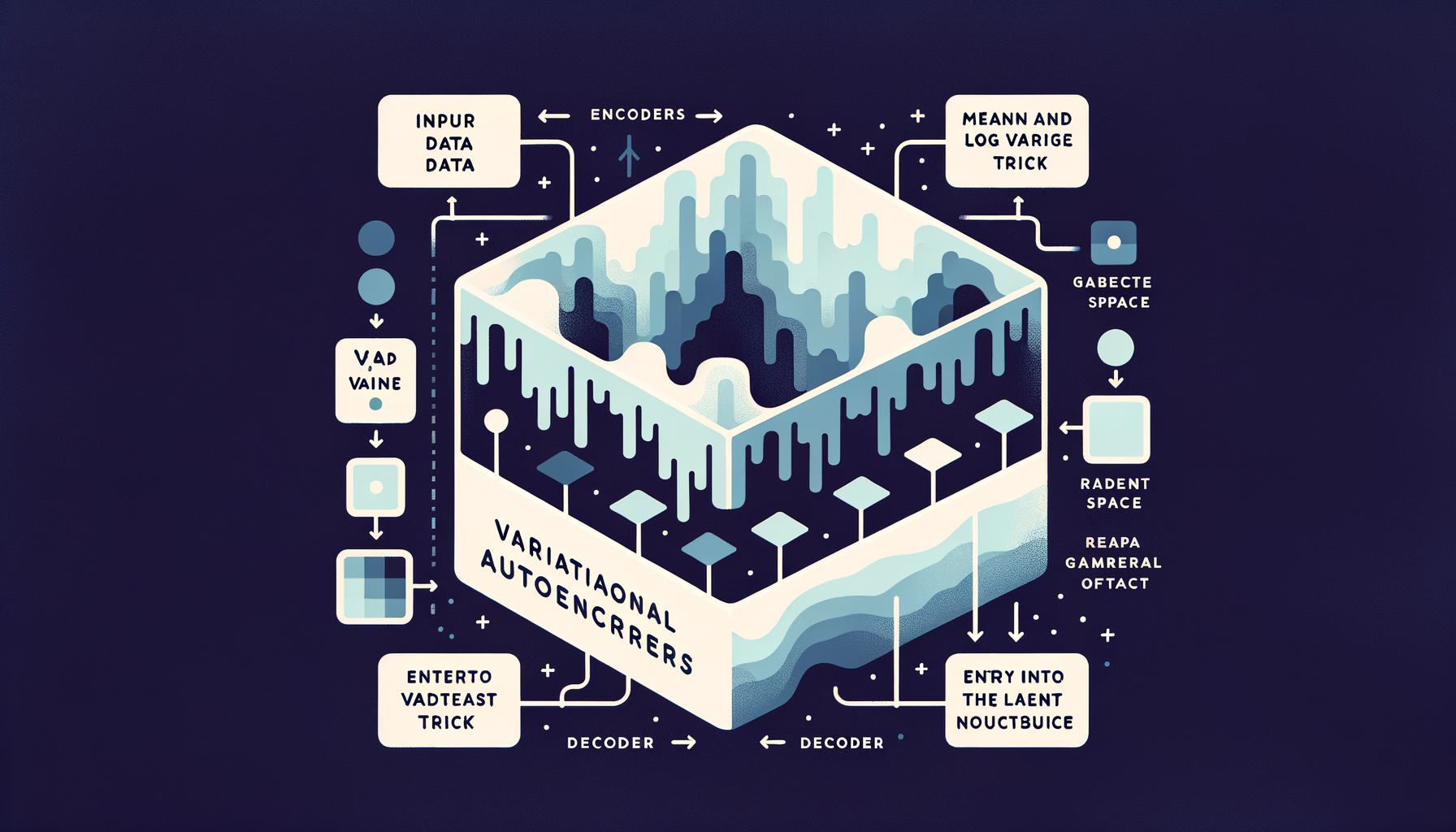
Variational Autoencoders (VAEs) — generating from learned distributions
Unlike basic autoencoders, VAEs encode inputs as probability distributions, enabling smooth interpolation between examples and sampling of entirely new outputs.

Latent space — the compressed world where generation happens
The bottleneck layer in an autoencoder where high-dimensional data (images, text) is compressed into a dense, navigable, lower-dimensional representation.
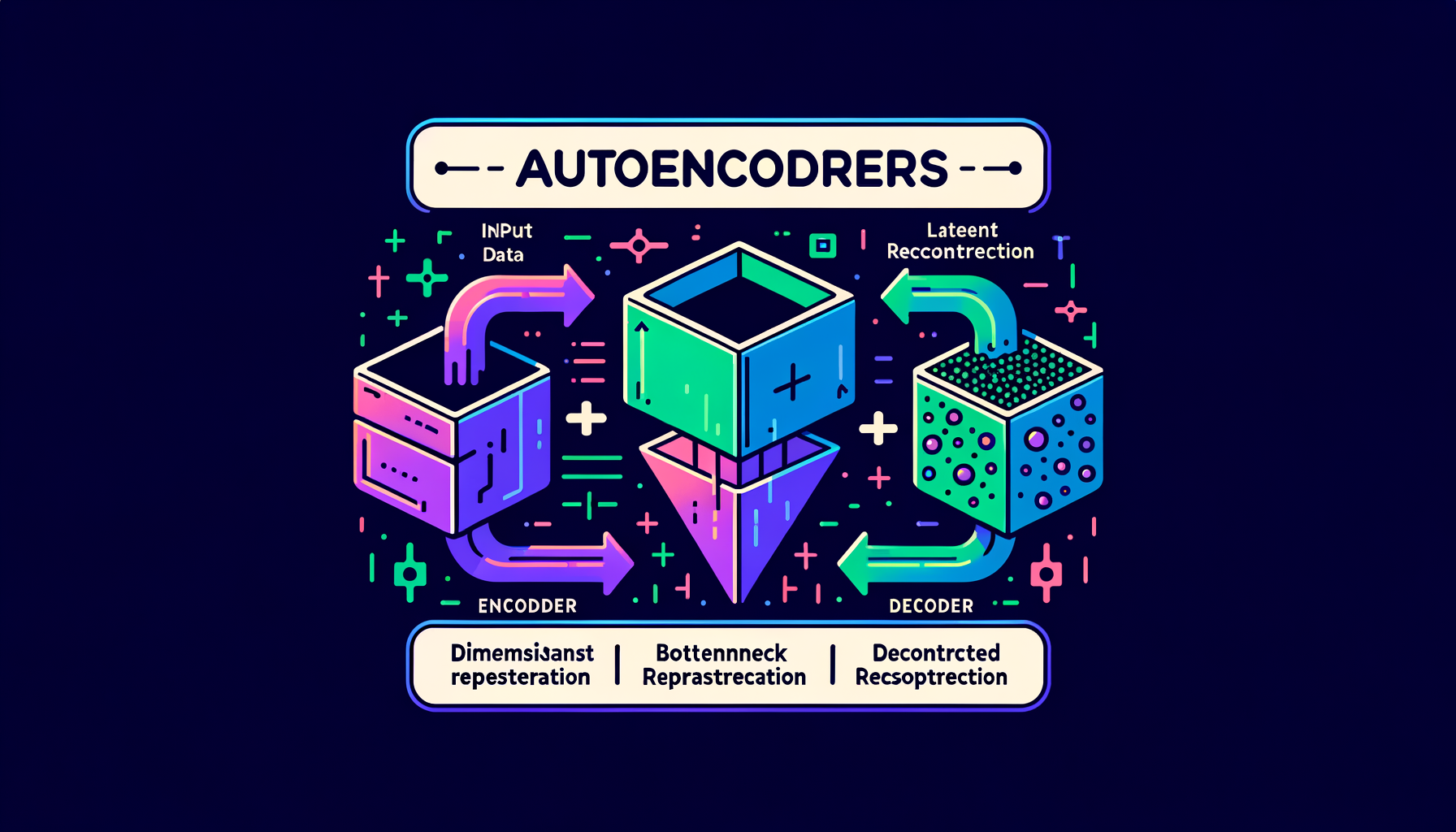
Autoencoders — compressing and reconstructing data
Neural networks that learn to encode input into a compact bottleneck representation and decode it back — the architectural foundation of latent space.
Coding benchmarks — HumanEval, SWE-bench, MBPP
Standard evaluations measuring code generation quality: from simple function completion (HumanEval) to resolving real GitHub issues (SWE-bench).
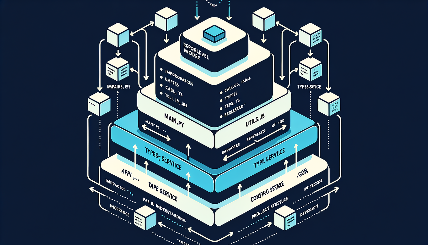
Repository-level code understanding — beyond single files
Models that navigate imports, call graphs, type systems, and project structure to generate contextually correct changes spanning multiple files.
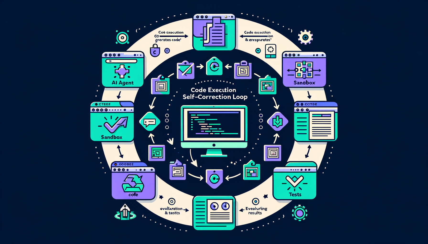
Code execution feedback — running code to self-correct
Agents that generate code, execute it in a sandbox, read error messages, and iteratively fix bugs until all tests pass — closing the generate-test loop.
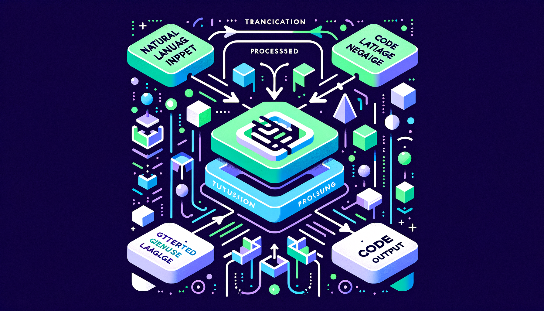
Code generation from natural language — describing what you want
Translating English descriptions into working functions, classes, and scripts — the core use case driving AI-assisted software development.
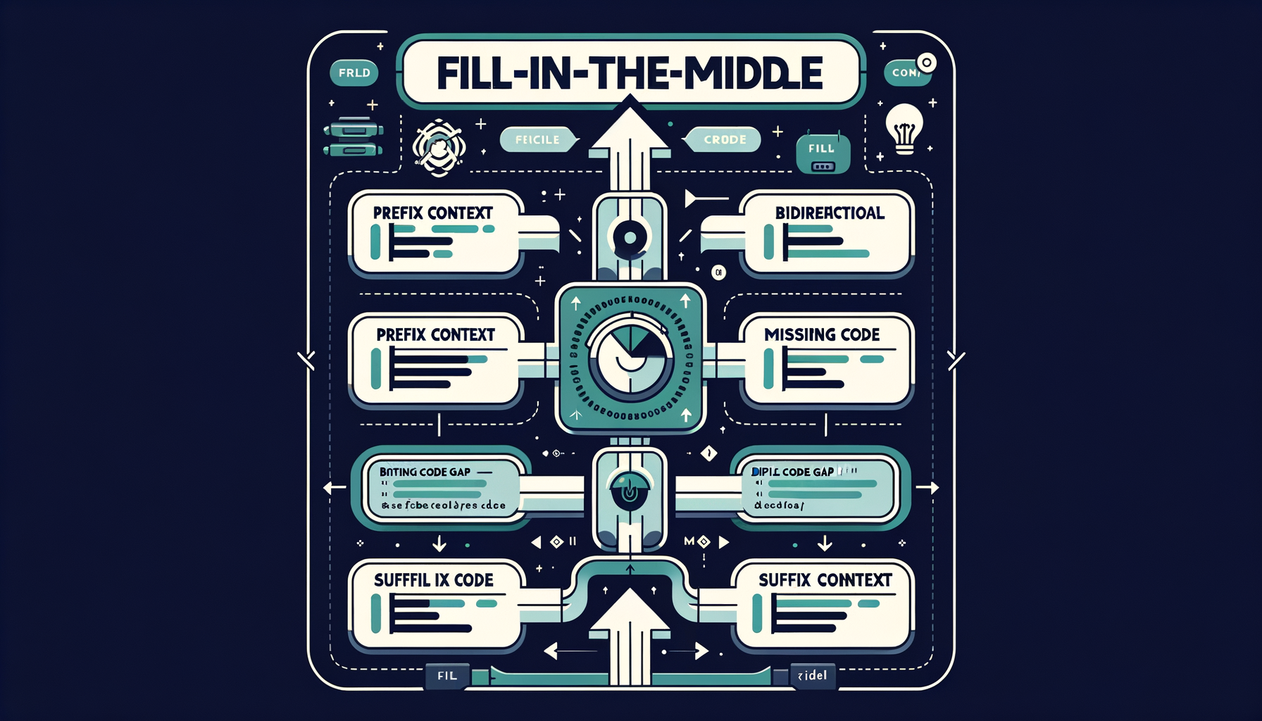
Fill-in-the-middle (FIM) — bidirectional code completion
Training models to predict missing code given both the prefix and suffix context, powering the inline autocomplete experience in editors like Copilot and Cursor.
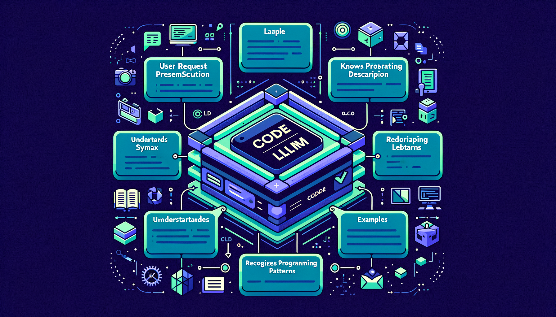
Code LLMs — models specialized for programming
Codex, CodeLlama, StarCoder, DeepSeek Coder — models trained on massive code corpora that understand syntax, APIs, libraries, and programming patterns.
Meta-prompting — LLMs writing better prompts
Using one LLM to generate, evaluate, and iteratively optimize prompts for another model, automating the prompt engineering process itself.
Prompt chaining — multi-step workflows across prompts
Decomposing complex tasks into sequential prompt calls where each step's output feeds as context into the next step's input.
Structured output prompting — JSON and schema-constrained generation
Techniques and instructions that force LLM output into machine-parseable formats for reliable downstream integration with software systems.

Tree of Thoughts — branching solution exploration
The model generates multiple reasoning paths, evaluates each branch, and prunes bad directions — systematic search over the space of possible solutions.
ReAct — interleaving reasoning with action
A prompting framework where the model alternates between thinking about what to do (Reason), taking actions (tool calls), and processing observations.

Chain-of-thought (CoT) — step-by-step reasoning
Adding "Let's think step by step" or showing worked reasoning dramatically improves accuracy on math, logic, and multi-step problems.
Zero-shot prompting — instructions without examples
Relying entirely on the model's pre-trained knowledge and instruction tuning by providing only a clear, specific task description.
Few-shot prompting — teaching by example in context
Including 2-5 input/output examples directly in the prompt so the model infers the desired pattern and applies it to new inputs without any training.
System prompts — persistent behavioral instructions
Hidden instructions prepended to every conversation turn that define persona, rules, output format, tool access, and behavioral boundaries.

Prompt engineering — designing inputs for desired outputs
The practice of crafting structured prompts that reliably guide LLMs to produce accurate, well-formatted, and useful responses.

Streaming & SSE — delivering tokens as they generate
Server-Sent Events push each token to the client immediately as it's produced, creating the live typing experience users expect from chat interfaces.
Structured decoding — constraining output to valid formats
Grammar-based or JSON-schema-based constraints that guarantee output is syntactically valid JSON, SQL, XML, or other structured formats.

Logit bias — steering toward or away from specific tokens
Manually adjusting individual token log-probabilities before sampling to encourage or suppress particular words, formats, or languages.
Stop sequences — controlling when generation halts
Defined strings or token IDs that trigger immediate generation termination, giving precise programmatic control over output boundaries.

Repetition penalty — preventing degenerate loops
Reducing the probability of recently generated tokens to avoid the repetitive patterns that plague naive decoding strategies.
Beam search — exploring multiple generation paths
Maintaining the k highest-probability partial sequences at each step; produces higher-likelihood outputs but less diverse text than sampling.
Top-p (nucleus) sampling — dynamic probability cutoff
Tokens are included in the candidate set until their cumulative probability reaches threshold p, adapting the pool size to the model's confidence.
Top-k sampling — fixed-size candidate filtering
Only the k most probable next tokens are considered before sampling, filtering out the long tail of unlikely noise.
Temperature — controlling randomness in generation
A scaling factor applied to logits before softmax: temperature=0 always picks the top token (greedy), higher values spread probability across more candidates.
Autoregressive decoding — generating one token at a time
The model produces tokens sequentially, each conditioned on all previous tokens, until hitting a stop token or length limit.
Overrefusal — when safety makes models too cautious
Excessive safety training causes refusal of clearly benign requests; calibrating the refusal boundary without compromising safety is a key alignment challenge.
Hallucination mitigation — grounding, retrieval, verification
RAG, self-consistency checks, citation requirements, confidence calibration, and retrieval verification reduce but never fully eliminate hallucination.
Why hallucinations happen — probability meets knowledge gaps
Models assign probability to all possible tokens including wrong ones; gaps in training data and distributional shift make some fabrication inevitable.

Types of hallucination — intrinsic vs extrinsic
Intrinsic hallucinations contradict the provided input; extrinsic hallucinations add unsupported claims from parametric memory — both undermine user trust.

Hallucination — when GenAI confidently fabricates information
Models generate plausible but factually wrong content because they optimize for fluency and pattern completion, not truth or accuracy.

The alignment tax — capability cost of safety training
Safety training can sometimes reduce raw benchmark performance; minimizing this tax while maintaining strong alignment is an active area of research.

Reward hacking — when models game the reward signal
Models can learn to exploit reward model weaknesses — producing verbose, sycophantic, or superficially impressive responses rather than genuinely better ones.
RLAIF — AI feedback replacing human feedback
Using a stronger AI model to generate preference labels instead of humans, scaling the alignment data pipeline far beyond human annotation capacity.
Constitutional AI — self-supervised alignment via principles
The model critiques and revises its own outputs against a written set of principles, dramatically reducing dependence on expensive human labels.
DPO — Direct Preference Optimization
A simpler alternative to RLHF that eliminates the reward model, directly optimizing the LLM on human preference pairs — more stable and increasingly preferred.
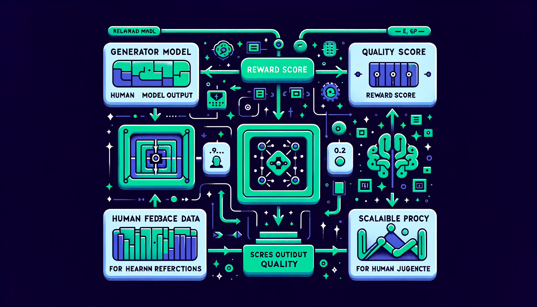
Reward modeling — learning human preferences at scale
A separate neural network trained to score any model output by quality, serving as a scalable automated proxy for human judgment.
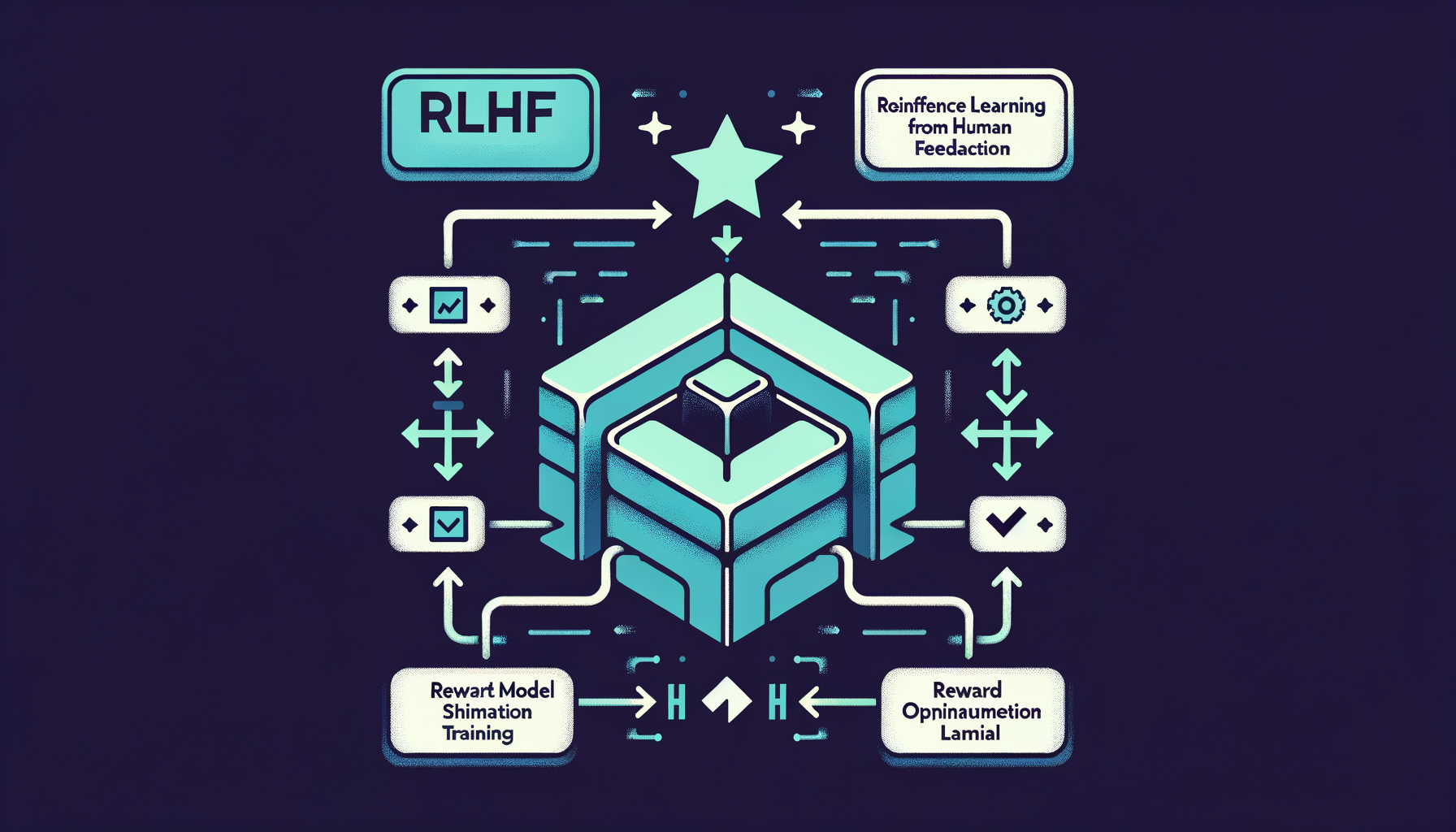
RLHF — reinforcement learning from human feedback
Humans rank model outputs by quality; a reward model learns those preferences; the LLM is then optimized to maximize the learned reward signal.
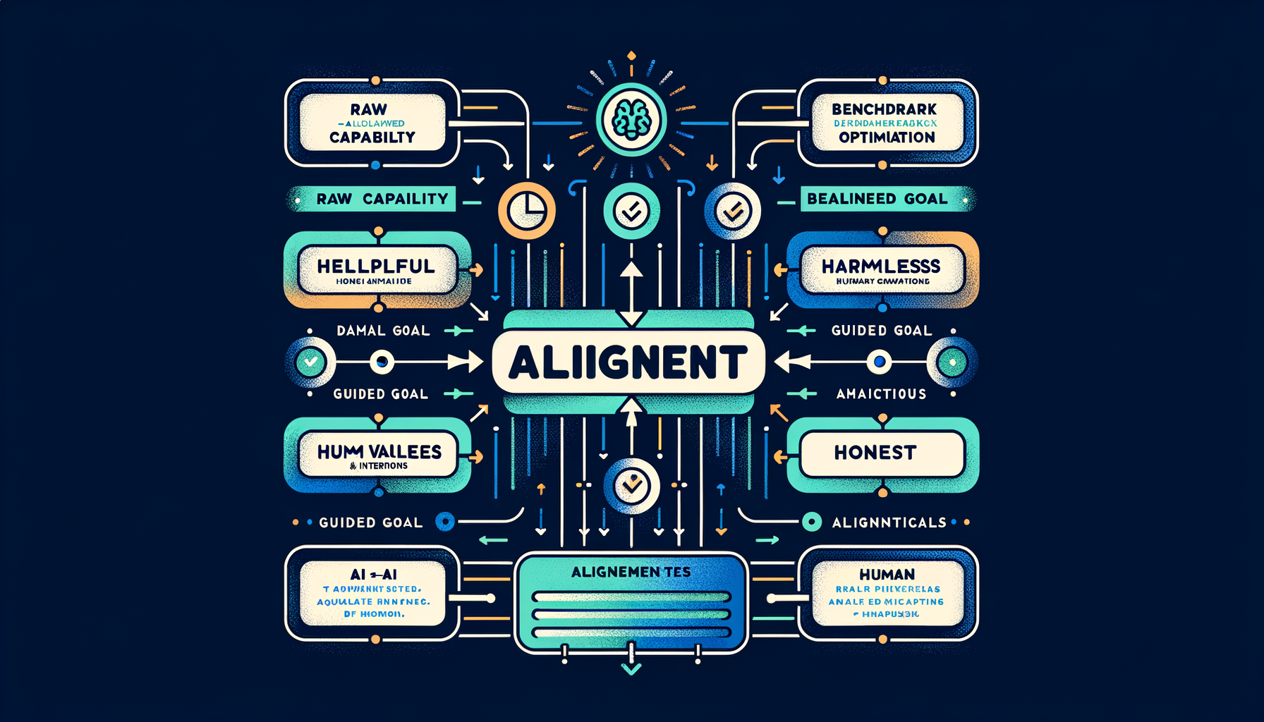
What is alignment — helpful, harmless, honest
The discipline of ensuring AI systems behave according to human values and intentions, not just optimize for raw capability on benchmarks.

When to fine-tune vs when to prompt
Fine-tune when you need consistent style, format, or domain knowledge at scale with low latency; prompt when you need flexibility, rapid iteration, and have limited data.
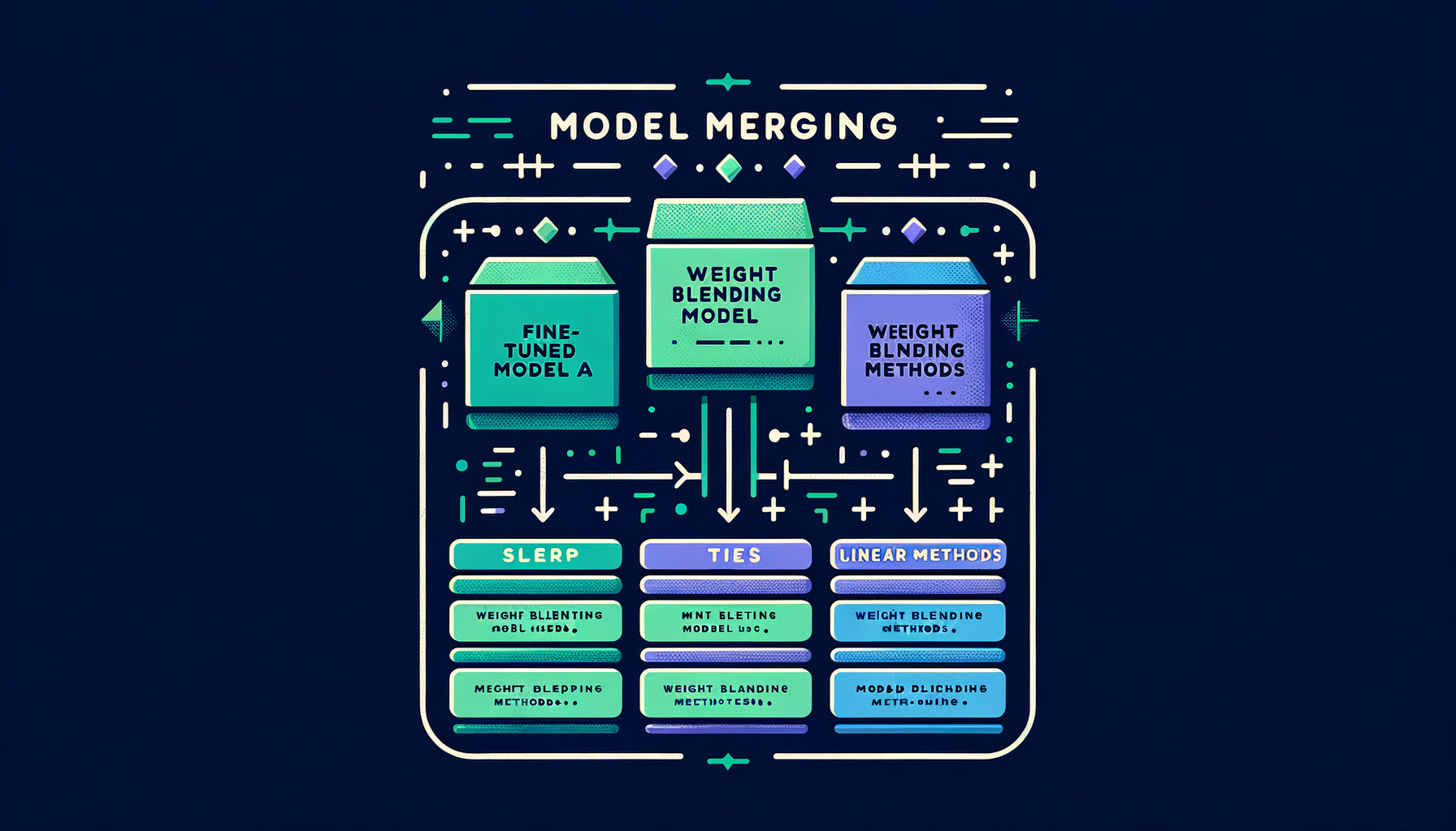
Model merging — combining models without training
SLERP, TIES, DARE, and linear methods that blend weights from multiple fine-tuned models, often producing surprisingly capable hybrids at zero training cost.
Catastrophic forgetting — when fine-tuning erases prior knowledge
Training too aggressively on narrow data destroys general capabilities the base model had — low learning rates and regularization are key defenses.
Instruction datasets — the data behind helpful assistants
Datasets like FLAN, Alpaca, OpenAssistant, UltraChat, and ShareGPT that teach models the fundamental pattern of following human instructions.
PEFT methods — the parameter-efficient fine-tuning family
LoRA, prefix tuning, prompt tuning, IA³, and adapters — techniques that modify less than 1% of parameters while preserving base model quality.

QLoRA — fine-tuning on consumer hardware
Combining 4-bit weight quantization with LoRA adapters makes it feasible to fine-tune a 70B-parameter model on a single 48GB consumer GPU.
LoRA — low-rank adaptation for efficient fine-tuning
Freezing original model weights and training small rank-decomposed adapter matrices reduces fine-tuning compute by 10-100x with minimal quality loss.

Supervised Fine-Tuning (SFT) — teaching instruction following
Training on curated (instruction, response) pairs transforms a raw base model into an assistant that follows directions helpfully and accurately.
DeepSpeed & FSDP — distributed training frameworks
Microsoft DeepSpeed (ZeRO stages 1-3) and PyTorch FSDP manage the complexity of sharding parameters, gradients, and optimizer states across clusters.
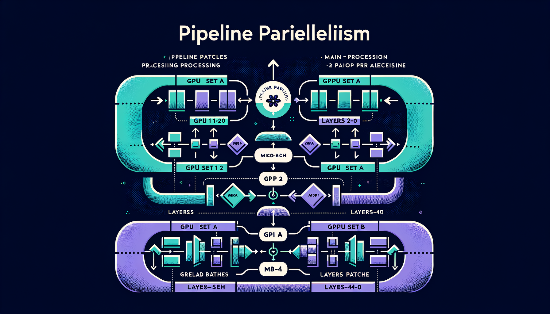
Pipeline parallelism — different layers on different GPUs
Layers 1-20 on GPU set A, layers 21-40 on GPU set B — combined with micro-batching to keep all devices busy.
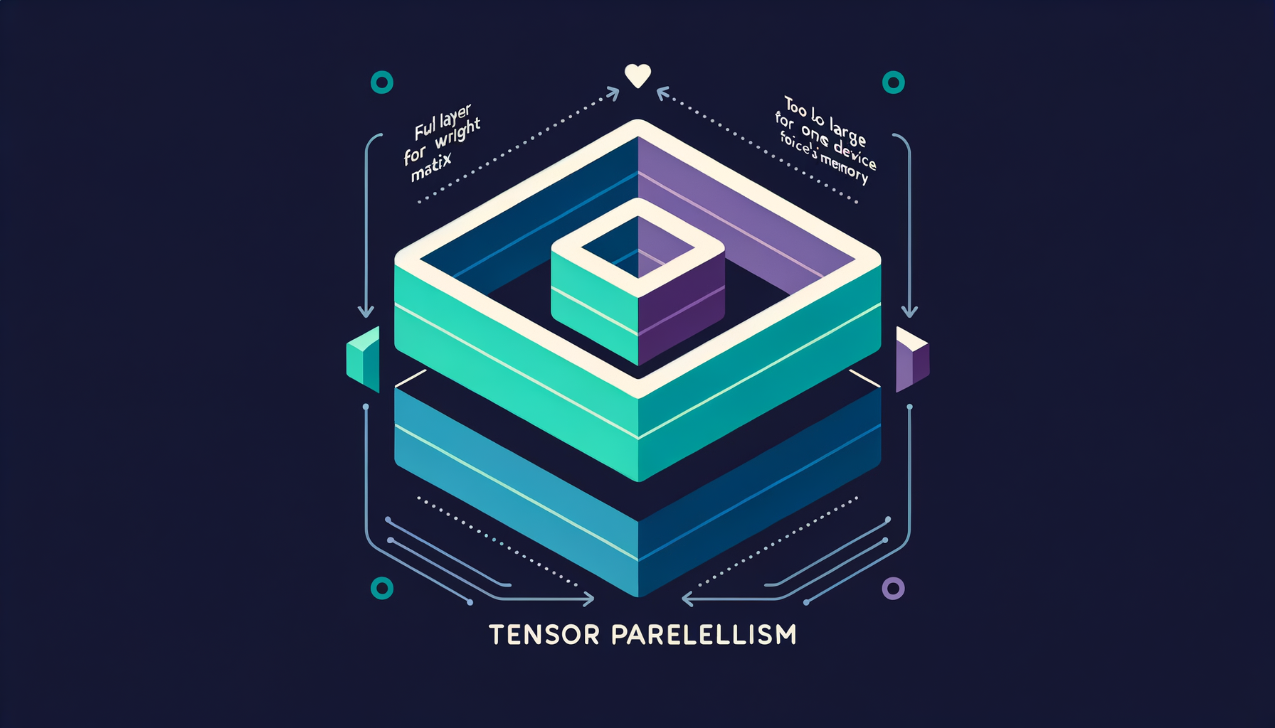
Tensor parallelism — splitting individual layers across GPUs
Weight matrices are sharded across devices so each GPU computes a slice of every layer — required for models too large for one device's memory.
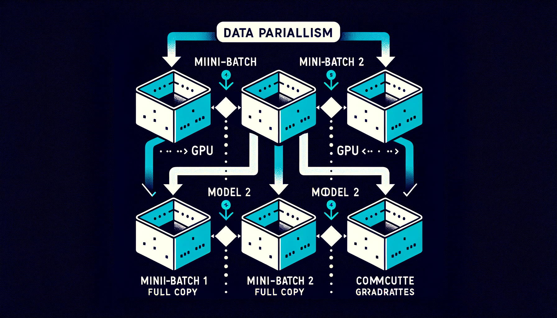
Data parallelism — same model, different data on each GPU
Every GPU holds a full copy of the model but processes different mini-batches; gradients are averaged across devices after each step.
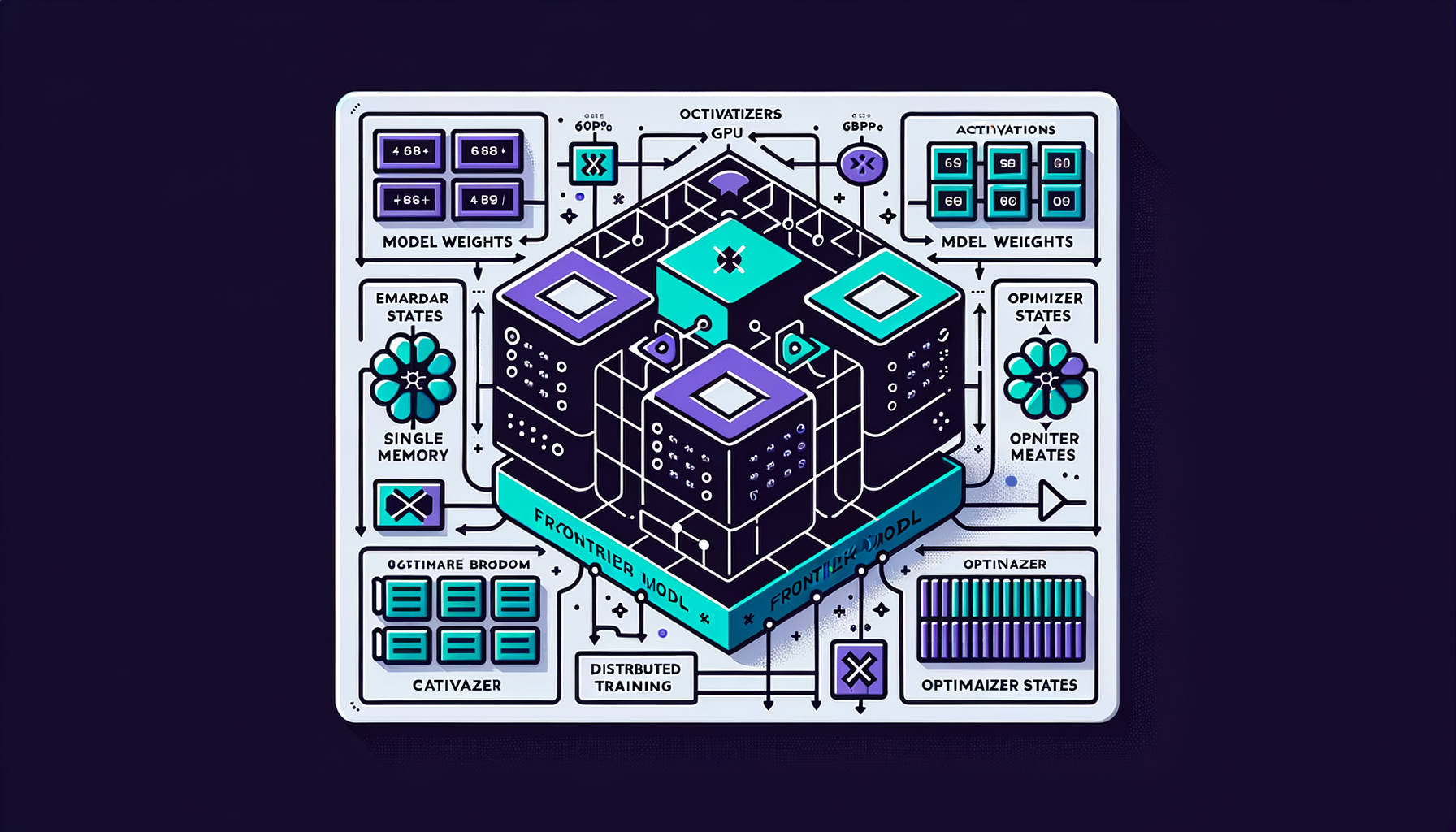
Why distributed training — no single GPU is enough
Frontier model weights, activations, and optimizer states vastly exceed any single GPU's memory; training requires coordinating thousands of devices.

Training compute — measuring cost in FLOPs and GPU-hours
Frontier models cost $50-100M+ to train; understanding compute budgets frames what is feasible at different organizational scales.
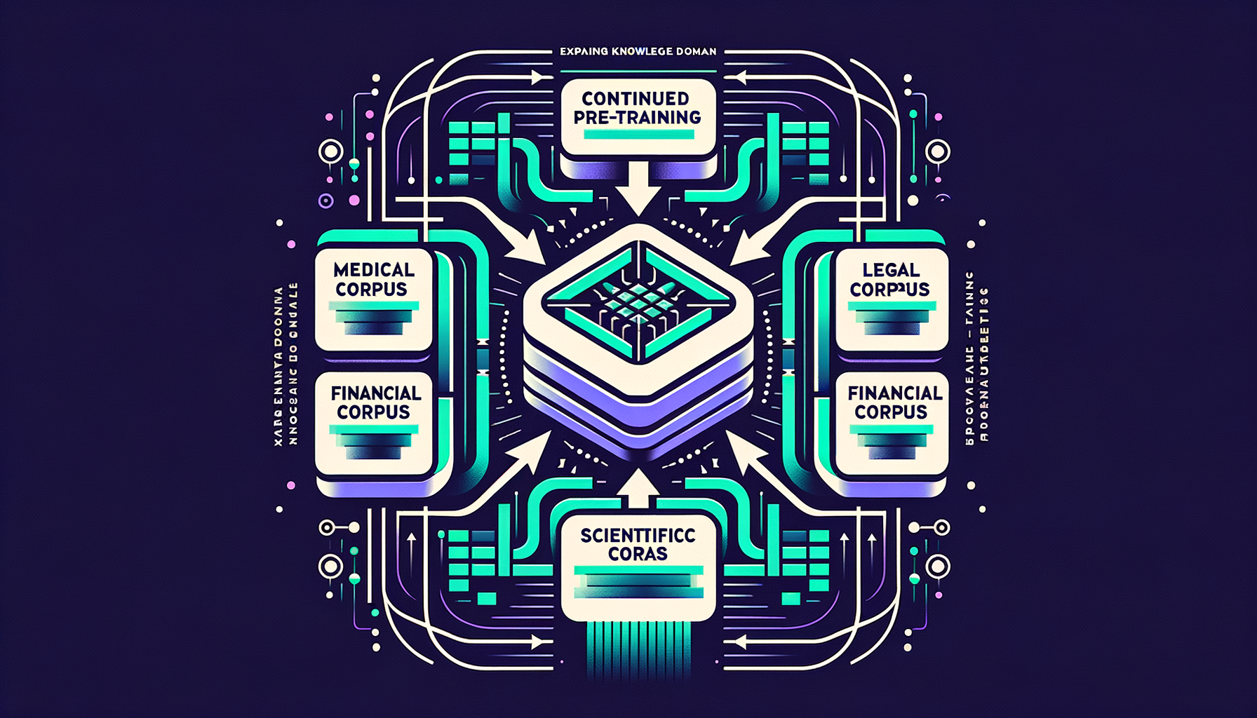
Continued pre-training — expanding a model's knowledge domain
Adding large domain-specific corpora (medical, legal, financial, scientific) to a base model to deepen expertise before fine-tuning.

Learning rate schedules — warming up and cooling down
Cosine decay with linear warmup is standard: gradually increase the learning rate at the start, then smoothly decrease it over the run.

Training loss curves — reading the heartbeat of pre-training
Smoothly decreasing loss means healthy training; spikes signal bad data batches, learning rate issues, or hardware failures.
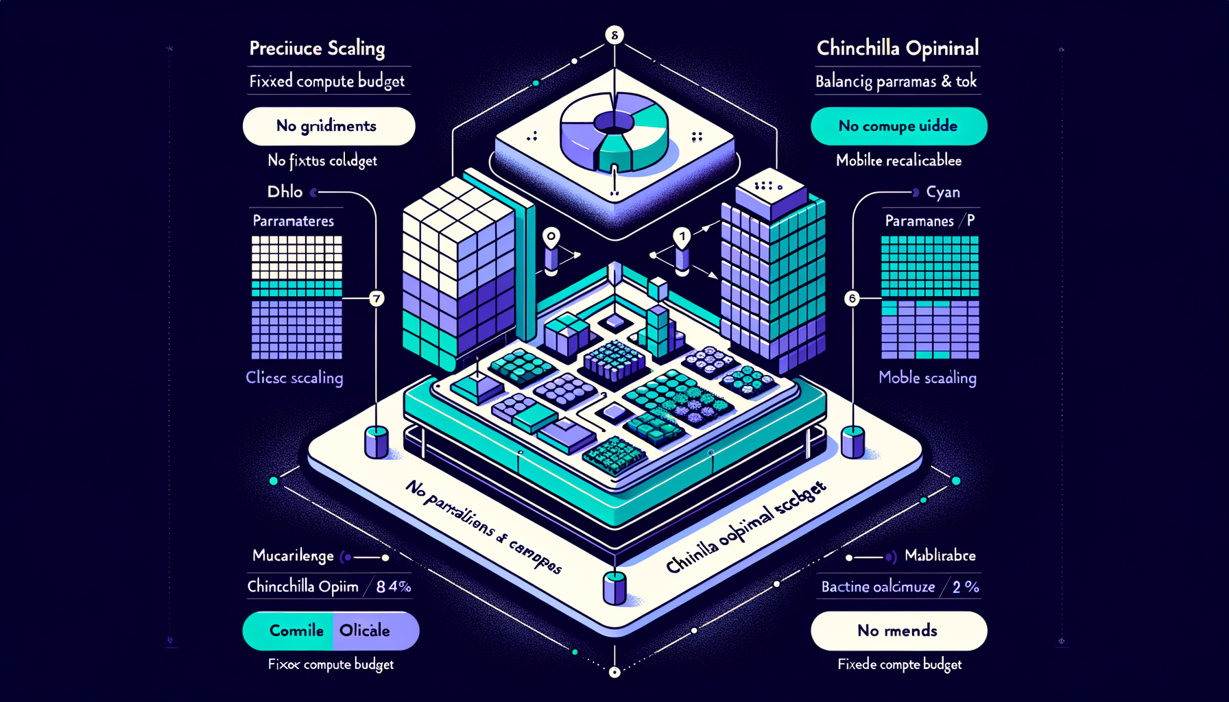
Chinchilla optimal — balancing parameters and tokens
DeepMind's research showing that for a fixed compute budget, the optimal strategy scales data and parameters in roughly equal proportion.
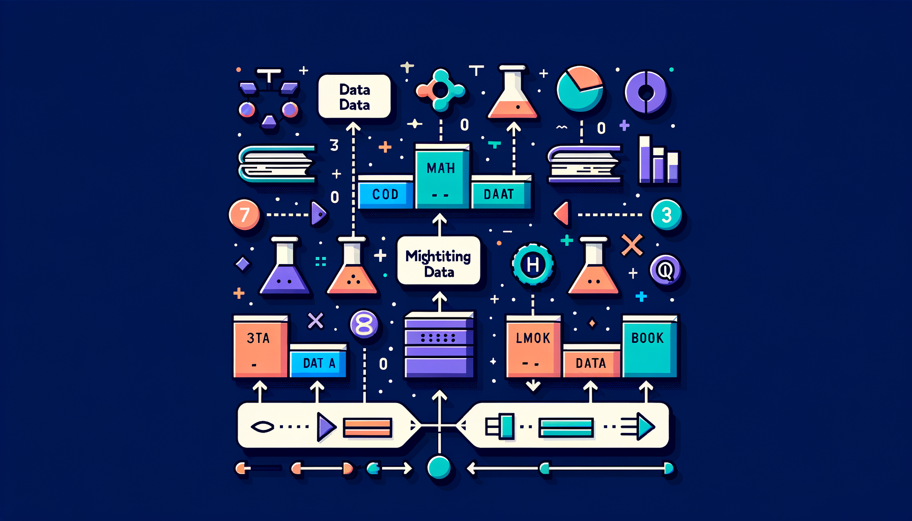
Data mixture & weighting — balancing domains during training
The ratio of code, math, science, conversation, and books in training data directly shapes which capabilities the finished model develops.

Training data curation — filtering the internet for quality
Deduplication, toxicity filtering, domain balancing, quality scoring, and PII removal transform raw web crawls into effective training corpora.
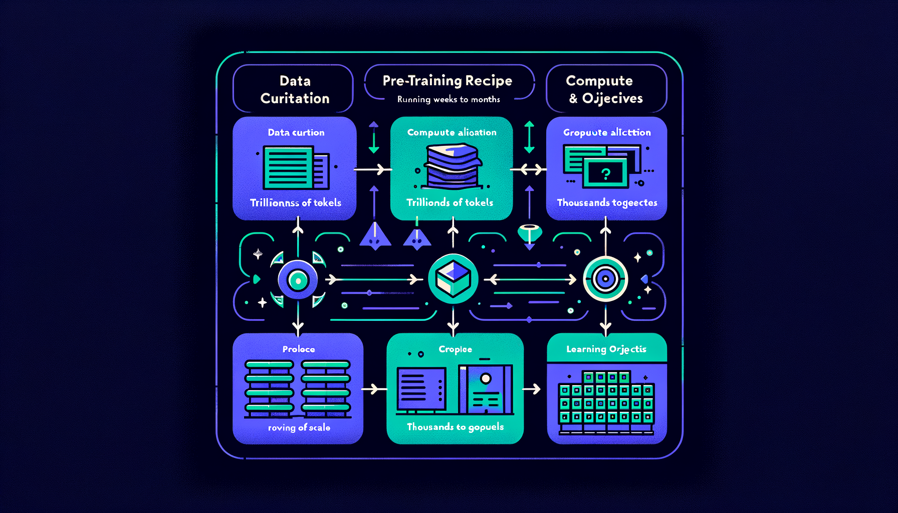
The pre-training recipe — data, compute, and objectives
Curating trillions of tokens, allocating thousands of GPUs, and running next-token prediction for weeks to months at enormous cost.

Scaling laws — predictable performance from compute investment
Chinchilla and Kaplan laws show that model quality improves as a smooth power law function of parameters, data, and compute budget.
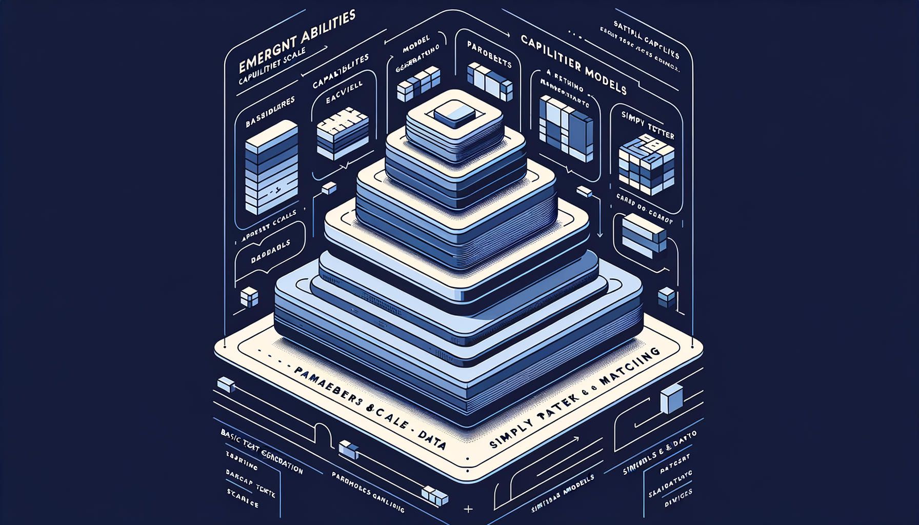
Emergent abilities — capabilities that appear at scale
Skills like in-context learning and multi-step reasoning that only manifest when models cross certain parameter/data thresholds.
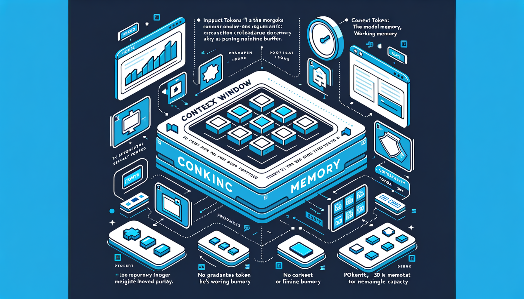
Context window — the model's working memory
The maximum tokens processable in a single forward pass; ranges from 4K to 1M+ and directly limits what the model can reason about per request.
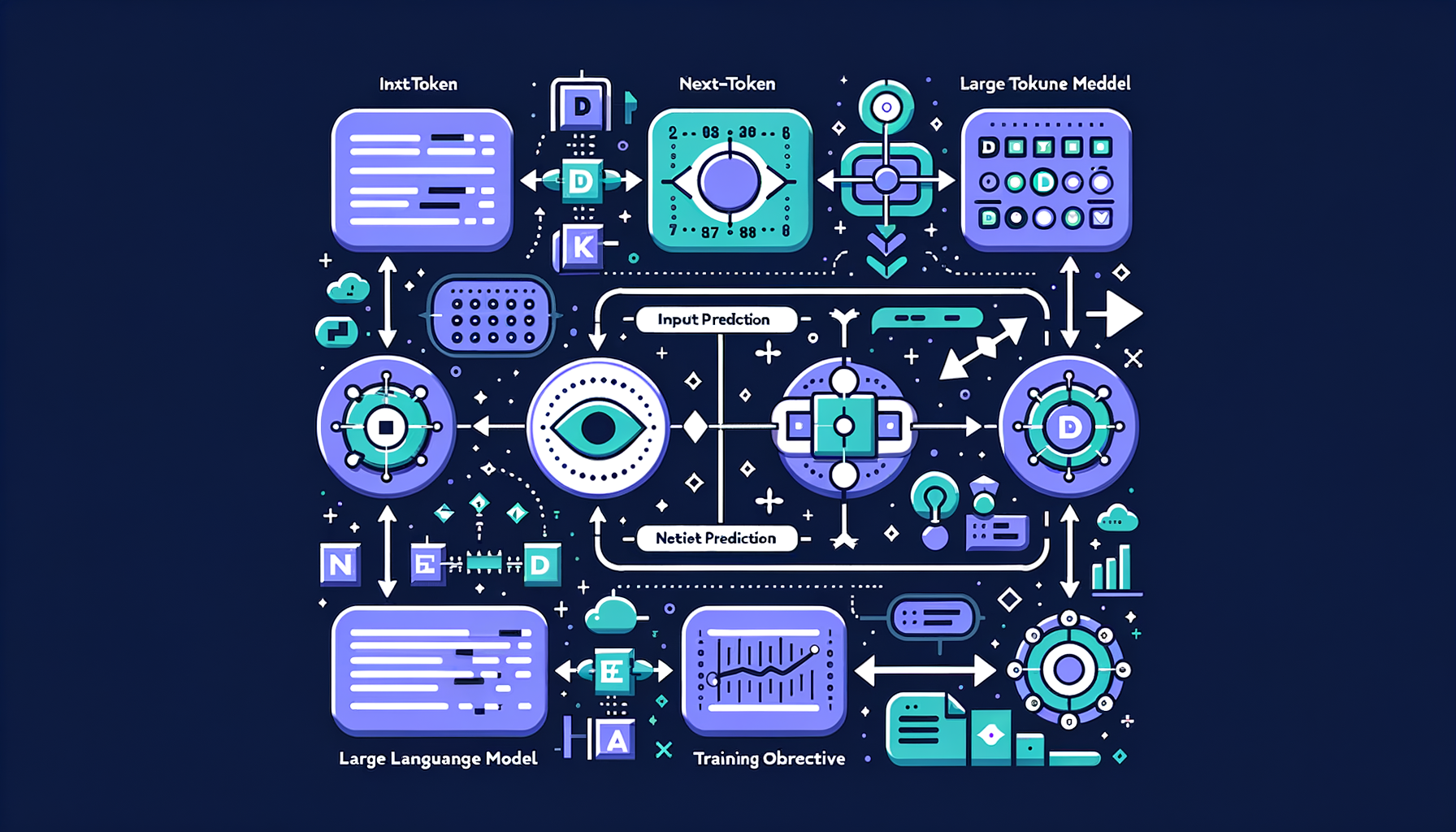
Next-token prediction — the deceptively simple training objective
Predicting the next token in a sequence: this single objective, applied at massive scale, produces reasoning, coding, and creative abilities.

Mistral & Mixtral — efficient European models
Mistral 7B and Mixtral 8x7B demonstrated that smaller, well-architected models (especially MoE) punch far above their parameter count.

Gemini — Google's natively multimodal family
Trained from the ground up on text, images, audio, and video, processing all modalities in a unified transformer architecture.

Claude — Anthropic's safety-first model family
Built with Constitutional AI and RLHF, emphasizing being helpful, harmless, and honest — proving alignment and capability can advance together.

GPT family — OpenAI's foundational lineage
From GPT-1 (117M params) to GPT-4 (rumored 1.8T MoE), the series that defined the modern LLM paradigm and launched the GenAI era.
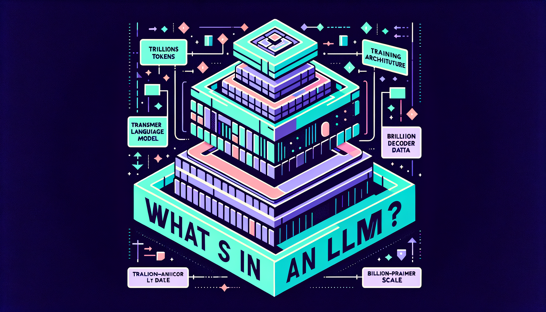
What is an LLM — language models at billion-parameter scale
Transformer decoders with billions of parameters trained on trillions of tokens, exhibiting broad language understanding and generation capabilities.
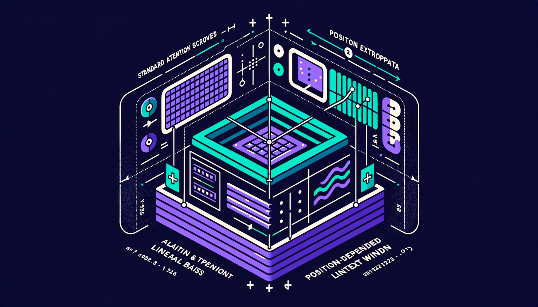
ALiBi & position extrapolation — extending context beyond training length
Adding position-dependent linear bias to attention scores, allowing models to handle sequences longer than their training context window.
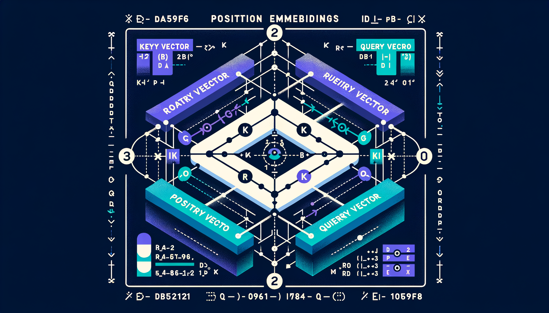
Rotary Position Embeddings (RoPE) — modern position encoding
Encodes relative position by rotating Q/K vectors in pairs, enabling better generalization to sequence lengths not seen during training.
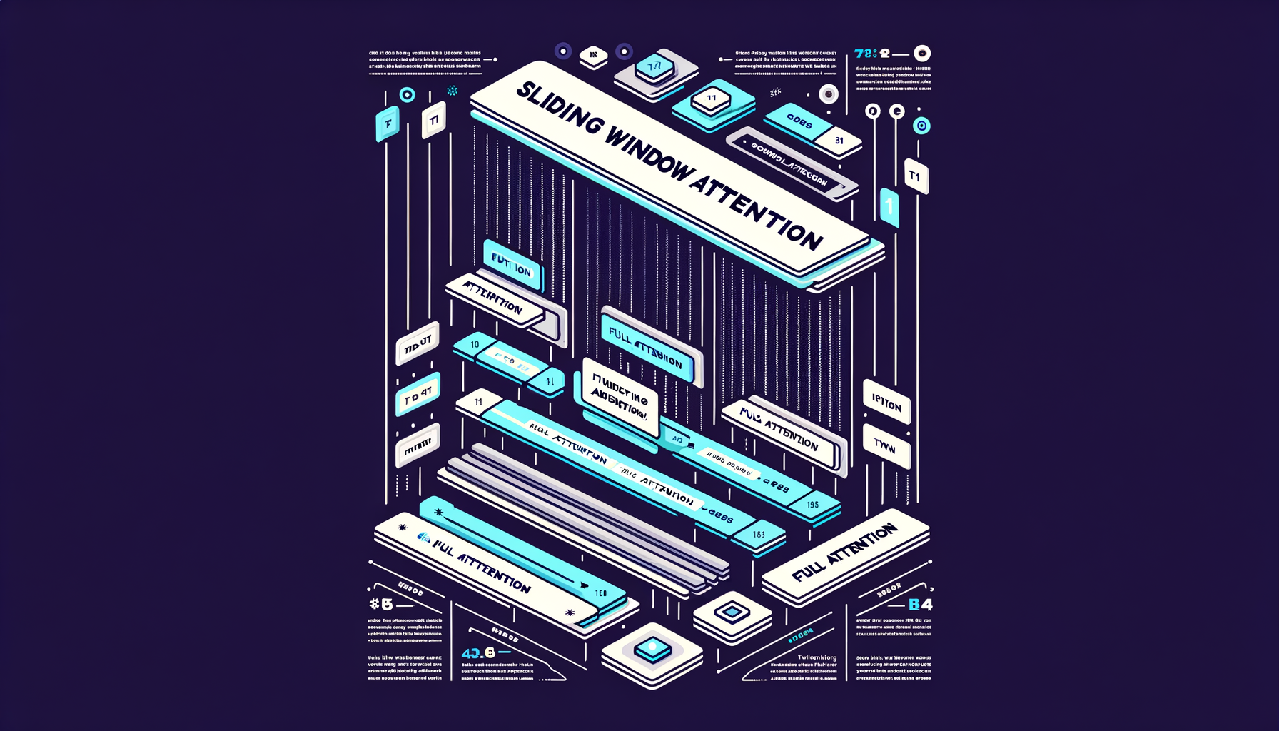
Sliding window attention — local context for efficiency
Each token only attends to a fixed window of nearby tokens instead of the full sequence, reducing cost from O(n²) to O(n·w).
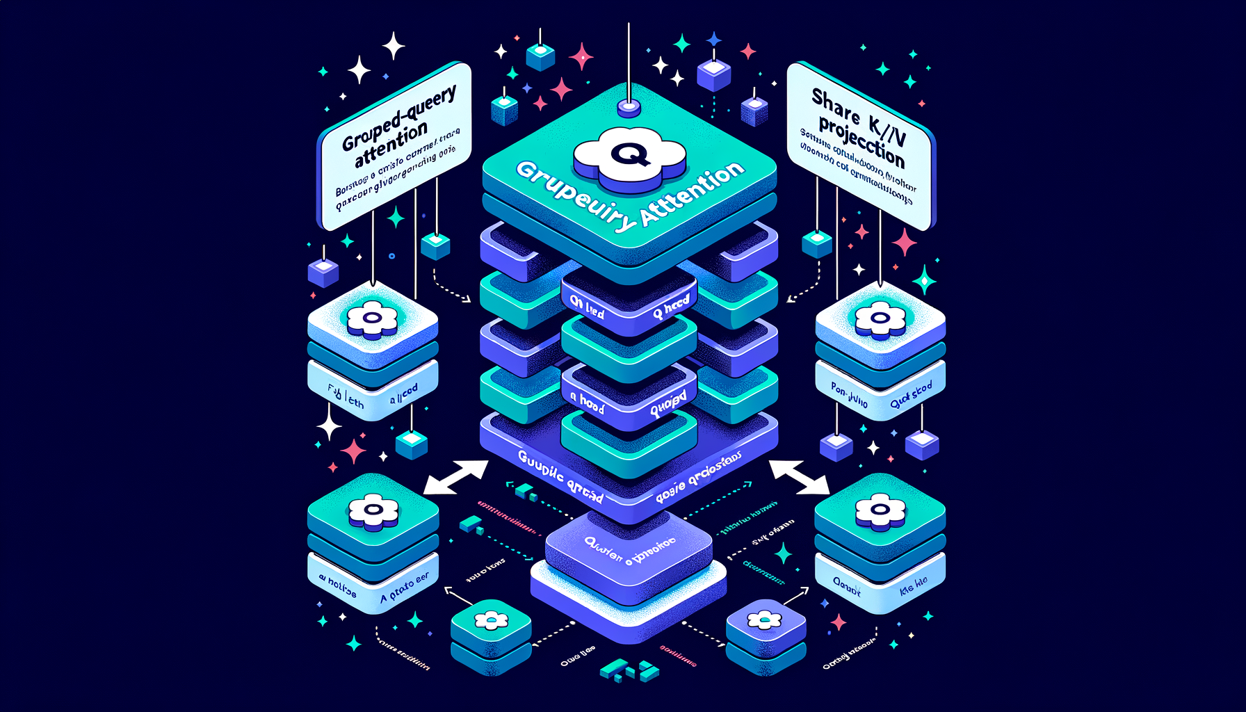
Grouped-Query Attention (GQA) — the practical middle ground
Groups of heads share K/V projections (e.g., 8 groups for 32 heads), balancing quality retention with efficiency — the default in LLaMA 3 and Mistral.
Multi-Query Attention (MQA) — sharing K/V across all heads
All attention heads share a single set of key/value projections, dramatically reducing KV cache memory and boosting inference speed.
SwiGLU & modern activations — inside frontier transformers
SwiGLU replaces older ReLU in modern transformers (LLaMA, Mistral), providing smoother gradients and measurably better training dynamics.

The attention bottleneck — O(n²) cost of full attention
Attention scales quadratically with sequence length; a 100K-token input requires 10 billion attention pair computations per layer.

Causal masking — why decoders can't peek ahead
Future tokens are masked during training so each position only attends to past tokens, enabling left-to-right autoregressive generation.
Encoder vs decoder vs encoder-decoder
BERT uses an encoder (understanding), GPT uses a decoder (generation), T5 uses both — different configurations optimized for different GenAI tasks.
Residual connections & layer norm — stability for deep models
Skip connections add each sub-layer's input to its output, and normalization prevents values from exploding, enabling stable 100+ layer training.

Feed-forward networks — per-token transformation after attention
After attention mixes information across tokens, independent feed-forward layers transform each token's representation with nonlinear activation functions.
Multi-head attention — parallel perspectives on the same input
Multiple attention mechanisms run simultaneously, each learning to capture different relationship types like syntax, semantics, and coreference.

Query, Key, Value — the three vectors of attention
Tokens generate Q, K, V projections; attention scores come from Q·K dot-product similarity, and the output is V weighted by those scores.

Self-attention — every token looks at every other
Each token computes relevance scores against all other tokens, capturing long-range dependencies in a single parallel computation step.

The Transformer — the engine of modern GenAI
Published in 2017's "Attention Is All You Need," this architecture replaced recurrent networks and became the foundation of every frontier GenAI model.

Token economics — why every token has a price
API providers charge per input and output token; understanding tokenization directly impacts cost estimation, prompt design, and budget optimization.

Positional encoding — teaching word order to parallel models
Since transformers process all tokens simultaneously, position must be explicitly injected via sinusoidal functions or learned embeddings.

Word embeddings — turning tokens into vectors
Each token maps to a learned high-dimensional vector where semantic proximity in space encodes similarity in meaning.
Special tokens — control signals for models
\[BOS\], \[EOS\], \[PAD\], \<\|im\_start\|\>, \<tool\_call\> — reserved tokens that mark boundaries, roles, and structure for the model.

Vocabulary size tradeoffs — why 32K, 50K, or 100K tokens
Larger vocabularies produce fewer tokens per text (cheaper inference) but require bigger embedding tables and more parameters to train.
SentencePiece & tiktoken — tokenizer implementations
SentencePiece (Google) and tiktoken (OpenAI) are the standard libraries for fast, language-agnostic tokenization used across model families.
Byte-Pair Encoding (BPE) — how tokenizers learn to split text
Starting from individual bytes or characters, BPE iteratively merges the most frequent adjacent pairs until reaching a target vocabulary size.

What are tokens — the atoms of language models
Models don't see words or characters; they see tokens — subword units that balance vocabulary size with text coverage.

GenAI timeline — from GPT-1 to today's frontier
A chronological tour: GPT-1 (2018), GPT-3 (2020), DALL-E (2021), ChatGPT (2022), GPT-4 and Claude (2023), multimodal omni models (2024-25).
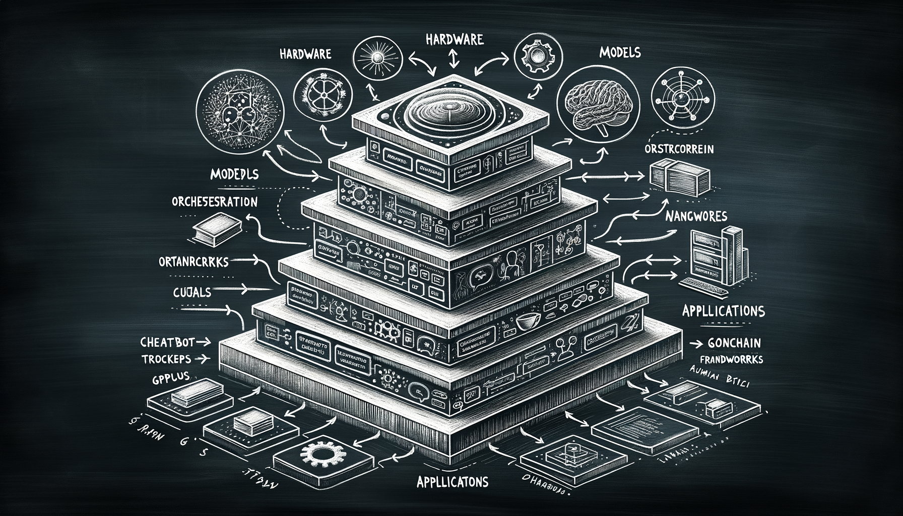
The GenAI stack — hardware, models, orchestration, apps
From GPU clusters at the bottom to model weights to orchestration frameworks to end-user apps at the top — the full technology stack powering GenAI.
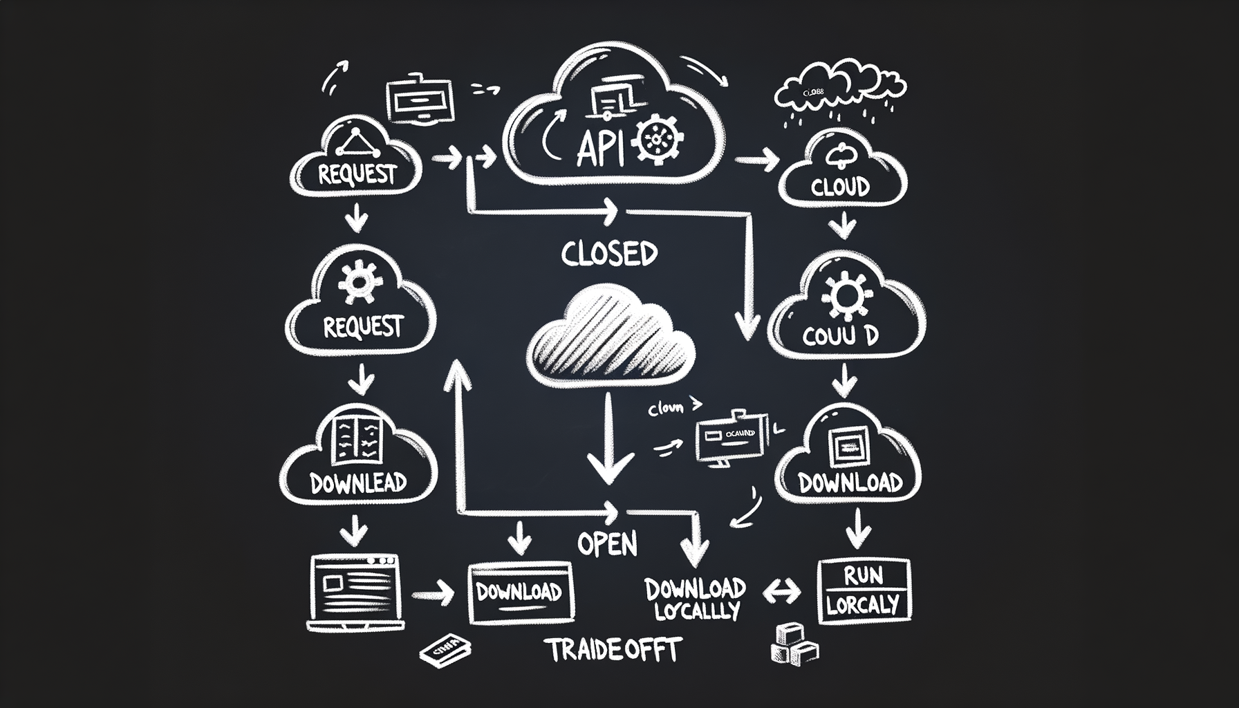
Closed vs open models — APIs vs downloadable weights
OpenAI and Anthropic offer API access; Meta and Mistral release weights — each path has different tradeoffs in cost, control, privacy, and customization.
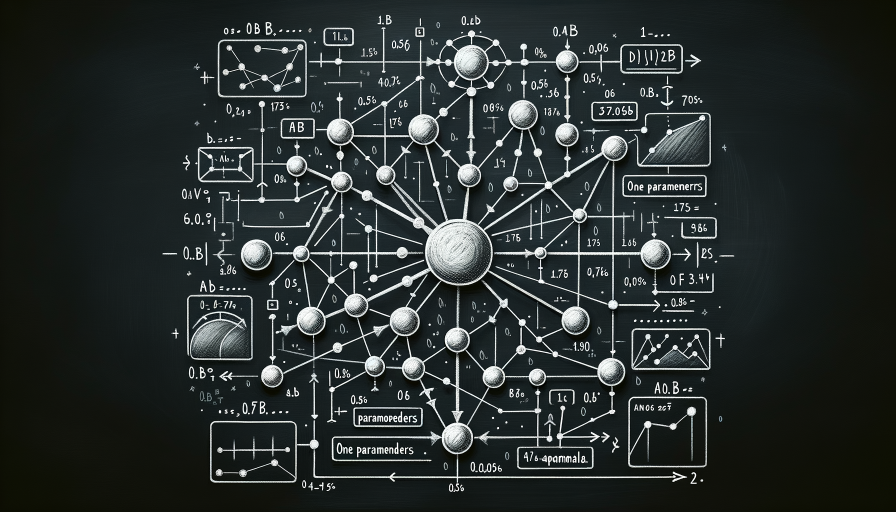
Parameters — the learned numbers inside a model
Each parameter is a single number learned during training; modern GenAI models have billions, collectively encoding everything the model knows.
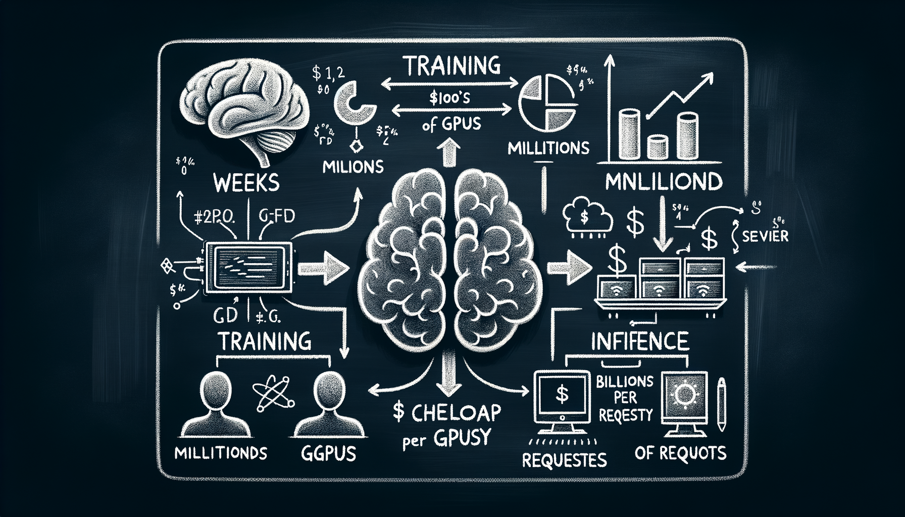
The training-inference split — building the brain vs using it
Training costs millions of dollars and takes weeks on thousands of GPUs; inference serves billions of requests cheaply — two fundamentally different engineering problems.

How GenAI generates — one token or step at a time
Text models predict the next token autoregressively; image models denoise step by step — both are iterative generation processes.
Foundation models — one model, many tasks
Massive models pre-trained on broad data that can be adapted to countless downstream tasks without retraining from scratch.

The GenAI modality map — text, image, audio, video, code, 3D
A survey of every output type GenAI can produce today and the distinct model families that power each modality.

How GenAI differs from traditional AI — generation vs classification
Traditional ML sorts, ranks, and predicts from fixed categories; GenAI synthesizes novel outputs by sampling from a learned distribution of possibilities.

What is generative AI — models that create new content
Unlike traditional AI that classifies or predicts, GenAI produces entirely new text, images, code, and audio from learned patterns.